Reinforcement Learning with Easy21
What is Reinforcement Learning?
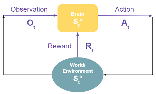
Reinforcement Learning (RL) is a form of machine learning that imitates the natural learning process of humans and other intelligent lifeforms.It is a powerful technique that can be used to create algorithms that are able to successfully operate a self-driving car or drone, manage power stations, or play games like Backgammon, Atari games, and Blackjack. Reinforcement learning provides a formalism for behavior. There is no supervised learning, only a reward signal. An RL agent tries to maximize the reward using data from the state of its environment and its own state. The agent operates according to a policy, which maps a state to an action. Based on a policy and given a state, an RL agent will choose an action.
The goal is to find the optimal policy that maximizes the accumulated reward.
There are different methods of finding optimal policies. To explore some of these approaches, I followed the RL lecture series taught by Dr. David Silver, computer science professor at the University College London. His introduction to reinforcement learning lecture series contains an assignment to build a game similar to Blackjack called Easy21. Below, I detail my solutions to Easy21 using Monte Carlo Simulation and Sarsa λ.
Lecture Series
Assignment link for the game rules
Building the Easy21 Environment
import random
import numpy as np

def draw():
    color = np.random.choice(['red', 'black'], p = [1/3, 2/3])
    number = random.randint(1,10)
    if color == 'red':
        number = - number
    return(number)

def init_zeros():
    return np.zeros([10,21,2])

def ep_greedy(N0, N, Q, p: int, d: int):

    epsilon = N0 / (N0 + np.sum(N[d - 1, p - 1, :]))
    explore = np.random.uniform(0, 1)

    if explore > epsilon:
        a = np.argmax(Q[d-1, p-1, :]) # get all actions and values

    else:
        a = random.choice([0,1]) # with probability epsilon, pick randomly
    return(a)

def step(a, state):
    r = 0
    d = state[0]
    p = state[1]

    if a == 0:
        p += draw()
        if p > 21 or p < 1:
            state = 'terminal'
            r = -1
        else:
            state[1] = p
            r = 0

    if a == 1:
        while d < 17 and d >= 1:
            d += draw()
        state = 'terminal'

        if d > 21 or d < 1 or d < p:
            r = 1
        elif d == p:
            r = 0
        elif d > p:
            r = -1

    return(state, r)
Monte Carlo Control
Monte Carlo simulation is a form of model-free prediction, meaning it has no knowledge of any pre-existing Markov Decision Processes (MDP) for transitions/rewards. MDP's formally describe an environment where the environment is fully observable by the state. MC methods learn directly from k episodes of experience. In Easy21 an episode is a game. The basic idea is that the value of a state/action is the empirical mean of the total discounted return.
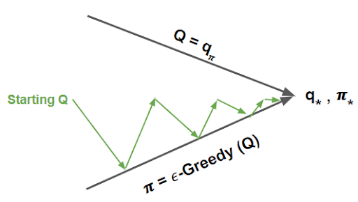
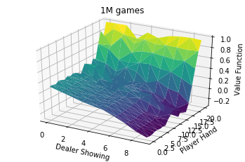
We want to learn the action-value function Q(s,a) from episodes of experience under policy, pi. To do this, we will use Monte Carlo estimation in control to approximate and find our optimal policy. The idea is to repeatedly evaluate and improve our policy to better estimate Q.
Under an epsilon greedy policy, we have action = argmaxa in A(Q(s,a)) with an exploration threshold denoted by epsilon, meaning with some probability epsilon we randomly choose an action. With MC, we run through an entire episode and then use the outcome reward to update our Q. This update effectively changes our policy. By changing our policy and evaluating after each episode, we eventually converge to our optimal policy and value function.
MC Control Python
import random
import pickle
import numpy as np
import pandas as pd
from utils.game_actions import *

def update_Q(N, Q, G, state_actions):
    for sa in state_actions:
        Q[sa] = Q[sa] + (1/N[sa])*(G - Q[sa])
    return Q

num_games = 100000
# Create Q(S,A)
Q = init_zeros()
# N_0 for epsilon
N0 = 100
# Create N state/action counter matrix thing
N = init_zeros()


for game in range(num_games):

    #initialize game
    p = random.randint(1,10)
    d = random.randint(1,10)

    state_actions = []

    G = 0
    state = [d,p]

    while state is not 'terminal':

        # get epsilon greedy action
        a = ep_greedy(N0, N, Q, p, d)

        # update N(S,A)
        N[d-1,p-1, a] += 1
        state_actions.append((d-1,p-1,a))

        # take one step in the game. Returns state and reward
        one_step = step(a, state)

        # update episode state
        state = one_step[0]

        # if state is terminal, end episode
        if state == 'terminal':
            reward = one_step[1]
            G += reward
        else:
            d = state[0]
            p = state[1]
            G += one_step[1]

    #update Q
    Q = update_Q(N, Q, G, state_actions)

pickle.dump(Q, open( "mc_QSA.p", "wb" )) # store true QSA

plot_mc(Q, num_games)
Plotting MC Control
def plot_mc(Q, num_games):
    # Get V
    V = np.amax(Q, axis=2)

    df = pd.DataFrame(V)
    plot_df = df.stack().reset_index()

    fig = plt.figure()
    ax = fig.gca(projection='3d')
    ax.plot_trisurf(plot_df['level_0'], plot_df['level_1'], plot_df[0], cmap=plt.cm.viridis, linewidth=0.1)

    # Set labels
    ax.set_xlabel('Dealer Showing')
    ax.set_ylabel('Player Hand')
    ax.set_zlabel('Value Function')
    ax.set_title('{} games'.format(num_games))
    ax.dist = 10.5

    plt.show()


Sarsa λ TD(λ) Control
Temporal difference learning is a model-free prediction method that bootstraps estimates of the action-value function Q and performs updates based on those estimates after each time step. Monte Carlo simulation must wait until the completion of an episode to get the cumulative returns Gt then average those returns to compute the value of a state and update Q. TD(λ) updates values based on bootstrapped estimates and therefore does not need to wait until the final outcome to make updates. TD(λ) is the averaging of n-backups and λ weights.
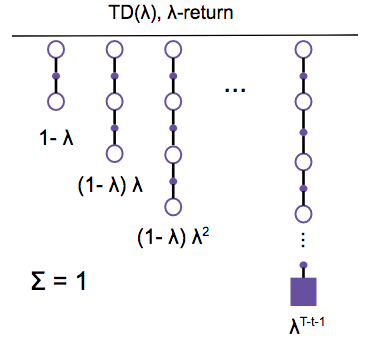
Sarsa λ is a method of TD control, so it employs the use of an eligibility trace to estimate the value of a state. An eligibility trace tells us how much credit/balance you should assign to each state/action. The main idea here is that when we make an update, we want to put more emphasis on the actions taken more recently that got us to where we are now. This is equivalent to saying we want to use more recent information to make a prediction about the future. Every time we get new information, we update our prediction.

Mathematically, this is implemented via the eligibility trace vector E(s,a). E(s,a) stores the decay factor for each state-action pair. The eligibility trace is applied to our TD error, δt, which is the difference between our prior estimate and the current estimate of Q.
SARSA λ Control Python
import random
import numpy as np
import pandas as pd
import itertools as it
import pickle
from utils.game_actions import *
from utils.plots import *

num_games = 10000
episode_mse_plot = np.zeros((len(lambdas), num_games))
lambda_mse_plot = np.zeros(len(lambdas))
N0 = 100
true_Q = pickle.load( open( "mc_QSA.p", "rb" ) )
lambdas  = np.arange(0, 1.1, 0.10).round(1)

for i, lmd in enumerate(lambdas):
    print('')
    # Create Q(S,A)
    Q = init_zeros()

    # Create N state/action counter matrix thing
    N = init_zeros()

    # Tracking wins per series of games with each lambda
    wins = 0

    # Games
    for ep in range(num_games):

        # Initialize game
        p = random.randint(1,10)

        d = random.randint(1,10)

        state_actions = []

        state = [d,p]

        E = init_zeros()

        # get epsilon greedy action
        a = ep_greedy(N0, N, Q, p, d)

        # Sample environments
        while state is not 'terminal':

            # take one step in the game
            one_step = step(a, state)

            # update episode state
            state = one_step[0]
            r = one_step[1]

            # update N(S,A)
            N[d-1,p-1, a] += 1


            state_actions.append((d-1,p-1,a))

            # if state is terminal, end episode
            if state == 'terminal':
                tderror = r - Q[d-1, p-1, a]

            else:
                d_prime = state[0]
                p_prime = state[1]

                a_prime = ep_greedy(N0, N, Q, p_prime, d_prime)

                tderror = (r + 1 * Q[d_prime-1, p_prime-1, a_prime]
                            - Q[d-1, p-1, a])

            # Update ESA
            E[d-1,p-1, a] += 1

            # Update QSA
            alpha = (1/N[d-1, p-1, a])
            Q = Q + E * tderror * alpha

            E = E * 1 * lmd

            if state != 'terminal':
                d = d_prime
                p = p_prime
                a = a_prime

        diff = Q - true_Q

        mse = np.sum(np.square(diff)) / 420
        episode_mse_plot[i, int(ep)] = mse

        if r == 1:
            wins += 1

        if ep % 1000 == 0:
            print('Episode: {}  Lambda: {}   MSE: {:.3f}'.format(ep, lmd, mse))

    lambda_mse_plot[i] = mse

    ratio = wins/(num_games) * 100
    print('TOTAL WINS: {}, {:.2f}%'.format(wins, ratio))


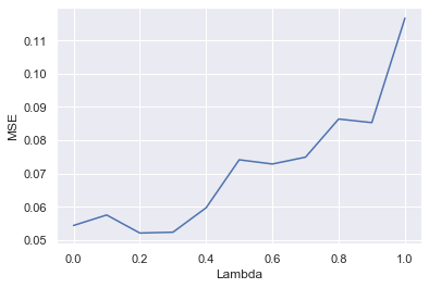
plot_final_lambda(lambda_mse_plot, lambdas)

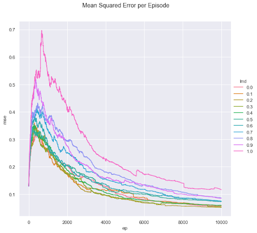
plot_mse_episodes(episode_mse_plot, lambdas)
Plotting Sarsa λ Control
def plot_final_lambda(lambda_mse_plot, lambdas):
    plt.plot(lambdas, lambda_mse_plot)
    plt.ylabel('MSE')
    plt.xlabel('Lambda')
    plt.show()

def plot_mse_episodes(episode_mse_plot, lambdas):
    names = ['lmd','ep']
    index = pd.MultiIndex.from_product([range(s) for s in episode_mse_plot.shape], names=names)
    df = pd.DataFrame({'mse': episode_mse_plot.flatten()}, index=index)['mse']
    df = df.reset_index(0).reset_index()
    df['lmd'] = df['lmd']/10
    m = sns.FacetGrid(df, hue="lmd", size=8, legend_out = True)
    m = m.map(plt.plot, "ep", "mse").add_legend()
    m.fig.suptitle('Mean Squared Error per Episode')
    plt.subplots_adjust(top=0.9)
    plt.show()
